股价绘图以及SVM/SVR策略
step1:前期准备,模块安装
1. 模块安装
激活环境后安装mpl_finance模块:
1 | (python36) $ pip install https://github.com/matplotlib/mpl_finance/archive/master.zip |
mpl_finance模块所包含的函数可参阅文档
安装tushare模块:1
(python36)$ pip install tushare
此处本人安装报错了,有提示报错原因,直接按其提示安装相关模块即可。1
(python36)$pip3 install module_name
2. 可视化数据
使用tushare的接口,get_h_data()获得一段时间内股价的复权数据。编辑器使用了jupyter,’%’是魔法函数。1
2
3
4
5
6
7
8
9import numpy as np
import tushare as ts
import matplotlib.pyplot as plt
#内置图像
%matplotlib inline
#生成svg矢量图格式的图形
%config InlineBackend.figure_format = 'svg'
data = ts.get_h_data('002337', start='2015-01-01', end='2015-12-16') #两个日期之间的前复权数据
plt.plot(data['close'])

除了折线图,我们加上蜡烛图(k线图),均线和成交量。首先我们需要安装talib用来计算均线。1
(python36)$ pip install talib
报错,安装失败。 具体报错信息如下: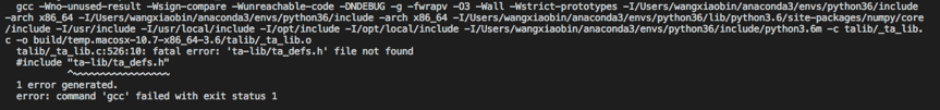
解决方案:https://stackoverflow.com/questions/49648391/how-to-install-ta-lib-in-google-colab
导入matlibplot.pyplot时出现错误: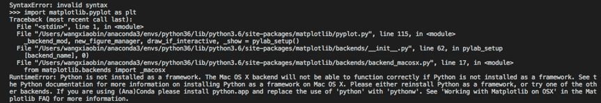
解决方案:
https://stackoverflow.com/questions/31373163/anaconda-runtime-error-python-is-not-installed-as-a-framework/41433353
使用tushare接口的get_k_data容易出现
整体代码如下:
1 | import numpy as np |

step2:数据处理
3. 通过tushare读取某只股票的两年数据并保存到本地。
1 | df = ts.get_h_data('002337', start='2015-01-01', end='2017-01-01') |
4. 利用pandas处理数据:提取特征,然后分类。
讲一下特征提取的方法:瞎几把提取( ̄▽ ̄)”:amt,volume,amt/volume,并且当(第三天的最高价-第一天的最低价)/第一天的开盘价 >= 0.02的时候设该行为1,否则置为-1。主要指导思想是证券和期货投资大师 威廉.欧奈尔的说法:个股的成交量能用来衡量个股供需双方的力量。当股价开始奔向近期新高,准备上一台阶的时候,此时的成交量应比最近几个月来的日平均成交量放大至少50%以上。1
2
3
4
5
6
7
8
9
10
11
12
13
14
15
16
17
18
19
20
21
22
23
24
25
26
27
28
29
30
31
32
33
34
35
36
37
38
39
40
41
42
43
44
45
46
47
48
49
50
51
52
53
54
55
56
57
58
59
60
61
62
63
64
65
66
67
68
69import pandas as pd
import os
def loadDataSetByPandas(filesname):
'''read csv files to a DataFrame
Args:
the list of the files
Returns:
merge all the files' data into a DataFrame exclude the rows 0
'''
dataFrame = pd.DataFrame()
for f in filesname:
dataFrame = dataFrame.append(pd.read_csv(f,header=0),ignore_index=True) #列名设为第0行,忽略index重复名
dataFrame = dataFrame[(dataFrame['amount']>0) & (dataFrame['volume']>0)] #处理缺失值0
return dataFrame
def listcsvFiles(_filepath):
''' list .csv files in specific filepath
Args:
_filepath: The path to list
Returns:
a list combined by the .csv file name under the path
'''
filecsv_list=[]
os.chdir(_filepath)
for root, dir, files in os.walk(_filepath):
for f in files:
if os.path.splitext(f)[1] == '.csv':
filecsv_list.append(f)
return filecsv_list
def count(_dataFrame):
'''统计DataFrame中label分别为1或-1的个数(要有好的分类效果,-1和1的个数最好持平)
Args:
Returns -> tuple: 例如:
return 1414, 1514
label: -1 , 1
'''
res = 0,0
minus1 = _dataFrame[_dataFrame['label'] == -1]
plus1 = _dataFrame[_dataFrame['label'] == 1]
res = len(minus1),len(plus1)
return res
def add_label(_dataFrame):
df = _dataFrame
df['Amt_div_Vol'] = df['amount'] / df['volume'] #给df增加一列Amt_div_Vol
df['label'] = (df['high'].shift(1)- df['low']) / df['close'] #增加一列label
df['label'] = df['label'].apply(lambda x : 1 if x >= 0.03 else -1) #修改label的值
'''
选取amt,volume,amt_div_vol作为三个特征,
label作为分类的标志
'''
df = df[['label','amount','volume','Amt_div_Vol']]
return df
if __name__ == '__main__':
root_dir = '/Users/wangxiaobin/Documents/git&hexo_blog/source/_posts/股价绘图以及SVM-SVR策略'
svm_train_dir = '/Users/wangxiaobin/Documents/git&hexo_blog/source/_posts/股价绘图以及SVM-SVR策略'
# svm_test_dir = '/Users/wangxiaobin/Desktop/大二下创新实践/作业4/作业4 Libsvm-股票数据分析/svm_test'
filecsv_list = listcsvFiles(root_dir)
df = loadDataSetByPandas(filecsv_list)
df = add_label(df)
df.to_csv('data_by_pandas.csv',header=None,index=None)
# 查看数据中正负类的个数
print(count(df))
5. 将提取的特征转成LIBSVM支持的格式
LIBSVM支持的格式长这个样子:
label 1:attr1 2:attr2 3:attr3 ···
我们直接使用convert.c编译成的convert把数据转成libsvm支持的格式。
1 | convert data_by pandas > /Users/wangxiaobin/Documents/git\&hexo_blog/source/_posts/股价绘图以及SVM-SVR策略/converted |
6. 数据归一化
由于每个特征的权重由其大小决定,为了保证每个特征的权重相同,我们必须把数据标准化、归一化。我们使用libsvm内置的工具svm-scale。1
/usr/local/lib/libsvm-3.22/svm-scale /Users/wangxiaobin/Documents/git\&hexo_blog/source/_posts/股价绘图以及SVM-SVR策略/converted > /Users/wangxiaobin/Documents/git\&hexo_blog/source/_posts/股价绘图以及SVM-SVR策略/scaled
step3:svm应用
7. 训练预测
1 | from svmutil import * |
结果如下:1
2
3
4
5
6
7
8
9
10➜ 股价绘图以及SVM-SVR策略 git:(master) ✗ python svmtrain.py
*..
WARNING: using -h 0 may be faster
*
optimization finished, #iter = 1152
nu = 0.685000
obj = -1095.381574, rho = -0.927679
nSV = 299, nBSV = 262
Total nSV = 299
Accuracy = 73.8636% (65/88) (classification)
8.优化C,gamma 参数后进行预测
1 | ➜ 股价绘图以及SVM-SVR策略 git:(master) ✗ python /usr/local/lib/libsvm-3.22/tools/grid.py scaled |
注意在使用grid.py前,查看是否需要修改grid.py源码中的路径,若与你的文件路径不符,请修正。否则会抛出无法找到文件的异常。
可以得到最优参数:c=128, g=8,然后,在第七步的基础上加上这个最优参数。最后得到1
2
3
4
5
6
7
8➜ 股价绘图以及SVM-SVR策略 git:(master) ✗ python svmtrain.py
.................*..................................*
optimization finished, #iter = 20659
nu = 0.642750
obj = -32444.879084, rho = -0.564842
nSV = 273, nBSV = 246
Total nSV = 273
Accuracy = 68.1818% (60/88) (classification)
你没有看错,准确率变低了(゚Д゚) ,还莫得思绪。
9.从混淆矩阵,ROC曲线中发现问题
我们知道,准确率(Accuracy)只是反映一个模型好坏的一个指标,但是光准确率一个指标不能较为全面地评价一个模型,因此为了更加客观评价一个模型,我们需要引入其他维度的指标:精确率(Precision)、召回率(Recall)以及以精确率和召回率为坐标轴的ROC曲线。这几个指标的具体含义,本文不展开(有时间在另写一片文章)。这里我发现使用Python的sklearn包能很方便的提供了我所需要的数学公式的接口,那么,我就开始用sklearn包来实现了。1
2
3#读入数据,
import pandas as pd
df = pd.read_csv('data_after_pandas.csv')
1 | # 确定特征集X和目标集y |
1 | # 把数据分为训练数据和测试数据 |
1 | from sklearn import svm |
观察predictions,发现预测结果都为1,很明显这个分类器没有起到很好的分类效果,虽然recall有1,但是accuracy_score和precision_score都只有0.672。指标的差异较大,且recall能有1可以说是非常不正常了,所以我们试着把混淆矩阵画出来以便理解recall等于1的结果。1
2
3
4
5
6
7
8
9
10
11
12
13
14
15
16
17
18
19
20
21
22
23
24
25
26
27
28
29
30
31
32
33
34
35
36
37
38
39
40
41
42
43
44
45
46
47
48
49
50
51
52
53
54
55
56
57
58
59
60
61# 混淆矩阵
import itertools
from sklearn.metrics import confusion_matrix
import matplotlib.pyplot as plt
import numpy as np
%matplotlib inline
%config InlineBackend.figure_format = 'svg'
def plot_confusion_matrix(cm, classes,
normalize=False,
title='Confusion matrix',
cmap=plt.cm.Blues):
"""
This function prints and plots the confusion matrix.
Normalization can be applied by setting `normalize=True`.
"""
if normalize:
cm = cm.astype('float') / cm.sum(axis=1)[:, np.newaxis]
print("Normalized confusion matrix")
else:
print('Confusion matrix, without normalization')
print(cm)
plt.imshow(cm, interpolation='nearest', cmap=cmap)
plt.title(title)
plt.colorbar()
tick_marks = np.arange(len(classes))
plt.xticks(tick_marks, classes, rotation=45)
plt.yticks(tick_marks, classes)
fmt = '.2f' if normalize else 'd'
thresh = cm.max() / 2.
for i, j in itertools.product(range(cm.shape[0]), range(cm.shape[1])):
plt.text(j, i, format(cm[i, j], fmt),
horizontalalignment="center",
color="white" if cm[i, j] > thresh else "black")
plt.tight_layout()
plt.ylabel('True label')
plt.xlabel('Predicted label')
# Compute confusion matrix
cnf_matrix = confusion_matrix(y_test, predictions)
np.set_printoptions(precision=2)
# Plot non-normalized confusion matrix
plt.figure()
plot_confusion_matrix(cnf_matrix, classes=['good','bad'],
title='Confusion matrix, without normalization')
# Plot normalized confusion matrix
plt.figure()
plot_confusion_matrix(cnf_matrix, classes=['good','bad'], normalize=True,
title='Normalized confusion matrix')
Confusion matrix, without normalization
[[ 0 40]
[ 0 82]]
Normalized confusion matrix
[[0. 1.]
[0. 1.]]


总算有点明白了按照Recall的公式: $R = \frac{TP}{TP+FN} $,其中$TP = 80,FN=0$,当然recall为1了。
总结 这个分类器是很失败的,把所有的实例都判断成了正类,其中究竟出了什么问题?在和同鞋的聊天中,他说的一点很中肯:数据的特征选择是重中之重。没选择好特征,分类器也就不能更好的工作了,可是难点也是特征选择,这些特征都是人工挑选出来的,无法得知特征的优劣,所以最后结果不符合要求也是可以理解的了。而对比本人此次实验,选的三个特征:成交量、成交总额、成交总额/成交量,也许并不太合适。我应该寻找一些更有具代表性的特征。